Stanford机器学习课程笔记1-Linear Regression与Logistic Regression

栏目：综合技术时间：2015-04-13 08:05:55

转载请注明出处: http://xiahouzuoxin.github.io/notes/

课程计划
Linear Regression与预测问题Locally Weighted Linear Regression
Logistic Regression与分类问题特点映照与过拟合(over-fitting)

Stanford机器学习课程的主页是： http://cs229.stanford.edu/

课程计划

主讲人Andrew Ng是机器学习界的大牛，创办最大的公然课网站coursera，前段时间还听说加入了百度。他讲的机器学习课程可谓每一个学计算机的人必看。全部课程的大纲大致以下：

Introduction (1 class) Basic concepts.
Supervised learning. (6 classes) Supervised learning setup. LMS. Logistic regression. Perceptron. Exponential family. Generative learning algorithms. Gaussian discriminant analysis.
Naive Bayes. Support vector machines. Model selection and feature selection. Ensemble methods: Bagging, boosting, ECOC.
Learning theory. (3 classes) Bias/variance tradeoff. Union and Chernoff/Hoeffding bounds. VC dimension. Worst case (online) learning. Advice on using learning algorithms.
Unsupervised learning. (5 classes) Clustering. K-means. EM. Mixture of Gaussians. Factor analysis. PCA. MDS. pPCA. Independent components analysis (ICA).
Reinforcement learning and control. (4 classes) MDPs. Bellman equations. Value iteration. Policy iteration. Linear quadratic regulation (LQR). LQG. Q-learning. Value function approximation. Policy search. Reinforce. POMDPs.

本笔记主要是关于Linear Regression和Logistic Regression部份的学习实践记录。

Linear Regression与预测问题

举了1个房价预测的例子，

Area(feet^2)	#bedrooms	Price(1000$)
2014	3	400
1600	3	330
2400	3	369
1416	2	232
3000	4	540
3670	4	620
4500	5	800

Assume：房价与“面积和卧室数量”是线性关系，用线性关系进行放假预测。因此给出线性模型， h_θ(x)?=?∑θ^Tx ，其中 x?=?[x₁,?x₂] , 分别对应面积和卧室数量。为得到预测模型，就应当根据表中已有的数据拟合得到参数 θ 的值。课程通过从几率角度进行解释（主要用到了大数定律即“线性拟合模型的误差满足高斯散布”的假定，通过最大似然求导就可以得到下面的表达式）为何应当求解以下的最小2乘表达式来到达求解参数的目的，

$J( heta)=frac{1}{2}sum_{i=1}^{m}(y_i-h_{ heta}(x_i))^2$

上述 J(θ) 称为cost function，通过 minJ(θ) 便可得到拟合模型的参数。

解 minJ(θ) 的方法有多种，包括Gradient descent algorithm和Newton's method，这两种都是运筹学的数值计算方法，非常合适计算机运算，这两种算法不但合适这里的线性回归模型，对非线性模型以下面的Logistic模型也适用。除此以外，Andrew Ng还通过线性代数推导了最小均方的算法的闭合数学情势，

$heta=(X^TX)^{-1}X^Told{y}$

Gradient descent algorithm履行进程中又分两种方法：batch gradient descent和stochastic gradient descent。batch gradient descent每次更新 θ 都用到所有的样本数据，而stochastic gradient descent每次更新则都仅用单个的样本数据。二者更新进程以下：

batch gradient descent
$heta_j:= heta_j+alphasum_{i=1}^{m}(y^{(i)}-h_{ heta}(x^{(i)}))x_j^{(i)}$
stochastic gradient descent
for i=1 to m
$heta_j:= heta_j+alpha(y^{(i)}-h_{ heta}(x^{(i)}))x_j^{(i)}$

二者只不过1个将样本放在了for循环上，1者放在了。事实证明，只要选择适合的学习率 α , Gradient descent algorithm总是能收敛到1个接近最优值的值。学习率选择过大可能造成cost function的发散，选择太小，收敛速度会变慢。

关于收敛条件，Andrew Ng没有在课程中提到更多，我给出两种收敛准则：

J小于1定值收敛
两次迭代之间的J差值，即|J-J_pre|<1定值则收敛

下面是使用batch gradient descent拟合上面房价问题的例子，

clear all;
clc

%% 原数据
x = [2014, 1600, 2400, 1416, 3000, 3670, 4500;...
    3,3,3,2,4,4,5;];
y = [400 330 369 232 540 620 800];

error = Inf;
threshold = 4300;
alpha = 10^(-10);
x = [zeros(1,size(x,2)); x];  % x0 = 0，拟合常数项
theta = [0;0;0]; % 常数项为0
J = 1/2*sum((y-theta'*x).^2);
costs = [];
while error > threshold
    tmp = y-theta'*x;
    theta(1) = theta(1) + alpha*sum(tmp.*x(1,:));
    theta(2) = theta(2) + alpha*sum(tmp.*x(2,:));
    theta(3) = theta(3) + alpha*sum(tmp.*x(3,:));
%     J_last = J;
    J = 1/2*sum((y-theta'*x).^2);
%     error = abs(J-J_last);
    error = J;
    costs =[costs, error];
end

%% 绘制
figure,
subplot(211);
plot3(x(2,:),x(3,:),y, '*');
grid on;
xlabel('Area');
ylabel('#bedrooms');
zlabel('Price(1000$)');

hold on;
H = theta'*x;
plot3(x(2,:),x(3,:),H,'r*');

hold on
hx(1,:) = zeros(1,20);
hx(2,:) = 1000:200:4800;
hx(3,:) = 1:20;
[X,Y] = meshgrid(hx(2,:), hx(3,:));
H = theta(2:3)'*[X(:)'; Y(:)'];
H = reshape(H,[20,20]);
mesh(X,Y,H);

legend('原数据', '对原数据的拟合', '拟合平面');

subplot(212);
plot(costs, '.-');
grid on
title('error=J(	heta)的迭代收敛进程');
xlabel('迭代次数');
ylabel('J(	heta)');

拟合及收敛进程以下：

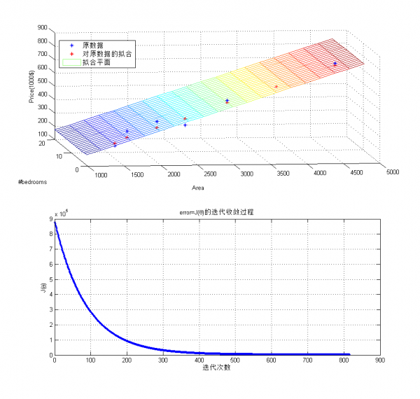
不论是梯度降落，还是线性回归模型，都是工具！！分析结果更重要，从上面的拟合平面可以看到，影响房价的主要因素是面积而非卧室数量。

很多情况下，模型其实不是线性的，比如股票随时间的涨跌进程。这类情况下， h_θ(x)?=?θ^Tx 的假定不再成立。此时，有两种方案：

建立1个非线性的模型，比如指数或其它的符合数据变化的模型
局部线性模型，对每段数据进行局部建立线性模型。Andrew Ng课堂上讲授了Locally Weighted Linear Regression，即局部加权的线性模型

Locally Weighted Linear Regression

$J( heta)=frac{1}{2}sum_{i=1}^{m}w^{(i)}(y^{(i)}-h_{ heta}(x^{(i)}))^2$

其中权值的1种好的选择方式是：

$w^{(i)}=old{exp}(-frac{(x^{(i)}-x)^2}{2 au^2})$

Logistic Regression与分类问题

Linear Regression解决的是连续的预测和拟合问题，而Logistic Regression解决的是离散的分类问题。两种方式，但本质殊途同归，二者都可以算是指数函数族的特例。

在分类问题中，y取值在{0,1}之间，因此，上述的Liear Regression明显不适应。修改模型以下

$h_{ heta}(x)=g( heta^Tx)=frac{1}{1+old{e}^{- heta^Tx}}$

该模型称为Logistic函数或Sigmoid函数。为何选择该函数，我们看看这个函数的图形就知道了，

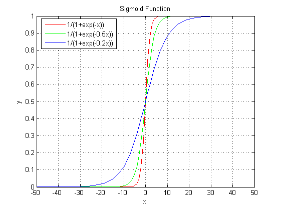
Sigmoid函数范围在[0,1]之间，参数 θ 只不过控制曲线的峻峭程度。以0.5为截点，>0.5则y值为1，< 0.5则y值为0，这样就实现了两类分类的效果。

假定 P(y?=?1|x;?θ)?=?h_θ(x) ， P(y?=?0|x;?θ)?=?1???h_θ(x) , 写得更紧凑1些，

$P(y|x; heta)=(h_{ heta}(x))^y(1-h_{ heta}(x))^{1-y}$

对m个训练样本，使其似然函数最大，则有

$old{max}L( heta)=old{max}prod_{i=1}{m}(h_{ heta}(x^{(i)}))^y^{(i)}(1-h_{ heta}(x^{(i)}))^{1-y^{(i)}}$

一样的可以用梯度降落法求解上述的最大值问题，只要将最大值求解转化为求最小值，则迭代公式1模1样，

$old{min}J( heta)=old{min}{-logold{L}( heta)}$

最后的梯度降落方式和Linear Regression1致。我做了个例子（数据集链接），下面是Logistic的Matlab代码，

function Logistic

clear all;
close all
clc

data = load('LogisticInput.txt');
x = data(:,1:2);
y = data(:,3);

% Plot Original Data
figure,
positive = find(y==1);
negtive = find(y==0);
hold on
plot(x(positive,1), x(positive,2), 'k+', 'LineWidth',2, 'MarkerSize', 7);
plot(x(negtive,1), x(negtive,2), 'bo', 'LineWidth',2, 'MarkerSize', 7);

% Compute Likelihood(Cost) Function
[m,n] = size(x);
x = [ones(m,1) x];
theta = zeros(n+1, 1);
[cost, grad] = cost_func(theta, x, y);
threshold = 0.1;
alpha = 10^(⑴);
costs = [];
while cost > threshold
    theta = theta + alpha * grad;
    [cost, grad] = cost_func(theta, x, y);
    costs = [costs cost];
end

% Plot Decision Boundary 
hold on
plot_x = [min(x(:,2))⑵,max(x(:,2))+2];
plot_y = (⑴./theta(3)).*(theta(2).*plot_x + theta(1));
plot(plot_x, plot_y, 'r-');
legend('Positive', 'Negtive', 'Decision Boundary')
xlabel('Feature Dim1');
ylabel('Feature Dim2');
title('Classifaction Using Logistic Regression');

% Plot Costs Iteration
figure,
plot(costs, '*');
title('Cost Function Iteration');
xlabel('Iterations');
ylabel('Cost Fucntion Value');

end

function g=sigmoid(z)
g = 1.0 ./ (1.0+exp(-z));
end

function [J,grad] = cost_func(theta, X, y)
% Computer Likelihood Function and Gradient
m = length(y); % training examples
hx = sigmoid(X*theta);
J = (1./m)*sum(-y.*log(hx)-(1.0-y).*log(1.0-hx));
grad = (1./m) .* X' * (y-hx);
end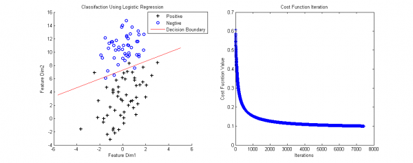

判决边界(Decesion Boundary)的计算是令h(x)=0.5得到的。当输入新的数据，计算h(x)：h(x)>0.5为正样本所属的类，h(x)< 0.5 为负样本所属的类。

特点映照与过拟合(over-fitting)

这部份在Andrew Ng课堂上没有讲，参考了网络上的资料。

上面的数据可以通过直线进行划分，但实际中存在那末种情况，没法直接使用直线判决边界(看后面的例子)。

为解决上述问题，必须将特点映照到高维，然后通过非直线判决界面进行划分。特点映照的方法将已有的特点进行多项式组合，构成更多特点，

$mapFeature=left[egin{array}{c}1 \ x_1 \ x_2 \ x_1^2 \ x_1x_2 \ x_2^2 end{array} ight]$

上面将2维特点映照到了2阶（还可以映照到更高阶），这便于构成非线性的判决边界。

但还存在问题，虽然上面方法便于对非线性的数据进行划分，但也容易由于高维特性造成过拟合。因此，引入泛化项应对过拟合问题。似然函数添加泛化项后变成，

$J( heta)=sum_{i=1}^{m}[-y^{(i)}log h(x^{(i)})-(1-y^{(i)})log(1-h(x^{(i)}))]+frac{lambda}{2}sum_{j=1}^n heta_j$

此时梯度降落算法产生改变，

$heta_j= heta_j+alphaleft[sum_{i=1}^{m}(y^{(i)}-h_{ heta}(x^{(i)}))x_j^{(i)}-lambda heta_j ight]$

最后来个例子，样本数据链接，对应的含泛化项和特点映照的matlab分类代码以下：

function LogisticEx2

clear all;
close all
clc

data = load('ex2data2.txt');
x = data(:,1:2);
y = data(:,3);

% Plot Original Data
figure,
positive = find(y==1);
negtive = find(y==0);
subplot(1,2,1);
hold on
plot(x(positive,1), x(positive,2), 'k+', 'LineWidth',2, 'MarkerSize', 7);
plot(x(negtive,1), x(negtive,2), 'bo', 'LineWidth',2, 'MarkerSize', 7);

% Compute Likelihood(Cost) Function
[m,n] = size(x);
x = mapFeature(x);
theta = zeros(size(x,2), 1);
lambda = 1;
[cost, grad] = cost_func(theta, x, y, lambda);
threshold = 0.53;
alpha = 10^(-1);
costs = [];
while cost > threshold
    theta = theta + alpha * grad;
    [cost, grad] = cost_func(theta, x, y, lambda);
    costs = [costs cost];
end

% Plot Decision Boundary 
hold on
plotDecisionBoundary(theta, x, y);
legend('Positive', 'Negtive', 'Decision Boundary')
xlabel('Feature Dim1');
ylabel('Feature Dim2');
title('Classifaction Using Logistic Regression');

% Plot Costs Iteration
% figure,
subplot(1,2,2);plot(costs, '*');
title('Cost Function Iteration');
xlabel('Iterations');
ylabel('Cost Fucntion Value');

end

function f=mapFeature(x)
% Map features to high dimension
degree = 6;
f = ones(size(x(:,1)));  
for i = 1:degree  
    for j = 0:i  
        f(:, end+1) = (x(:,1).^(i-j)).*(x(:,2).^j);
    end  
end
end

function g=sigmoid(z)
g = 1.0 ./ (1.0+exp(-z));
end

function [J,grad] = cost_func(theta, X, y, lambda)
% Computer Likelihood Function and Gradient
m = length(y); % training examples
hx = sigmoid(X*theta);
J = (1./m)*sum(-y.*log(hx)-(1.0-y).*log(1.0-hx)) + (lambda./(2*m)*norm(theta(2:end))^2);
regularize = (lambda/m).*theta;
regularize(1) = 0;
grad = (1./m) .* X' * (y-hx) - regularize;
end

function plotDecisionBoundary(theta, X, y)
%PLOTDECISIONBOUNDARY Plots the data points X and y into a new figure with
%the decision boundary defined by theta
%   PLOTDECISIONBOUNDARY(theta, X,y) plots the data points with + for the 
%   positive examples and o for the negative examples. X is assumed to be 
%   a either 
%   1) Mx3 matrix, where the first column is an all-ones column for the 
%      intercept.
%   2) MxN, N>3 matrix, where the first column is all-ones

% Plot Data
% plotData(X(:,2:3), y);
hold on

if size(X, 2) <= 3
    % Only need 2 points to define a line, so choose two endpoints
    plot_x = [min(X(:,2))-2,  max(X(:,2))+2];

    % Calculate the decision boundary line
    plot_y = (-1./theta(3)).*(theta(2).*plot_x + theta(1));

    % Plot, and adjust axes for better viewing
    plot(plot_x, plot_y)
    
    % Legend, specific for the exercise
    legend('Admitted', 'Not admitted', 'Decision Boundary')
    axis([30, 100, 30, 100])
else
    % Here is the grid range
    u = linspace(-1, 1.5, 50);
    v = linspace(-1, 1.5, 50);

    z = zeros(length(u), length(v));
    % Evaluate z = theta*x over the grid
    for i = 1:length(u)
        for j = 1:length(v)
            z(i,j) = mapFeature([u(i), v(j)])*theta;
        end
    end
    z = z'; % important to transpose z before calling contour

    % Plot z = 0
    % Notice you need to specify the range [0, 0]
    contour(u, v, z, [0, 0], 'LineWidth', 2)
end
end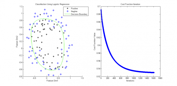

我们再回过头来看Logistic问题：对非线性的问题，只不过使用了1个叫Sigmoid的非线性映照成1个线性问题。那末，除Sigmoid函数，还有其它的函数可用吗？Andrew Ng老师还讲了指数函数族。

------分隔线----------------------------

上一篇 IP 分片丢失重传

下一篇 文件管理类NSFileManager常用操作

------分隔线----------------------------